
Pulse Calibration
The 1H 90o transmitter pulse can be determined with your own sample. Calibration of 13C or 15N decoupler pulses is most easily done using a sample that gives one sharp peak in a single scan, like the standard pulse calibration sample - 100 mM 13C methanol and 100 mM 15N urea in DMSO-d6. The 13C and 15N decoupler pulses are not very sample dependent and generally the default values read by "gpro" can be used.
Transmitter and decoupler
Transmitter and decoupler are terms used to refer to the different paths the radiofrequency pulses take. The transmitter is the path taken by pulses at the observe frequency, while the decoupler is the path taken by pulses at other frequencies. For example, in a 1H-13C HSQC experiment where the 1H frequency is the observe frequency, the 1H pulses are routed through the transmitter and the 13C pulses are routed through the decoupler. This is the typical arrangement for inverse detection probes. For experiments such as a 1D 13C experiment with 1H decoupling where 13C is the observe frequency, the 13C pulses are routed through the transmitter and the 1H decoupling pulses through the decoupler.
On Bruker instruments the routing of the pulses is defined by the pulse program. By default pulses are sent through the transmitter, which Bruker refers to as the f1 channel. If a pulse does not have a channel specified it will go through f1. Decoupler pulses are sent through the f2 or f3 channel when ":f2" or ":f3" appears after a pulse in the pulse program. By looking at the pulse program you can see which channels will be used for which pulses. When calibrating pulses you need to be aware of which channel you will be using in your experiments, so that you calibrate pulses using the appropriate routing.
Transmitter pulse
Background
At equilibrium the bulk magnetization of a sample inside a magnetic field aligns with the field, normally called the z axis. Detection is only possible for magnetization in the x-y plane orthogonal to the z axis. To maximize sensitivity the length of a pulse that rotates the magnetization 90o from the z axis to the x-y plane (left panel of figure below) needs to be calibrated. In multipulse experiments more than sensitivity is at stake. Efficient manipulation and transfer of the magnetization requires that the pulse lengths and power levels required for 90o and 180o pulses are known accurately.
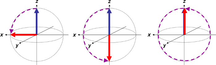
Vector diagrams showing the effects of 90o (left), 180o (center) and 360o pulses (right). The equilibrium bulk magnetization is shown as a blue arrow aligned along the z-axis. A pulse moves the magnetization vector along the trajectory shown by the dotted purple line to the position shown by the red arrow. Only the fraction of magnetization in the x-y plane is detectable.
Theoretically the 90o pulse could be determined by adjusting the pulse length until the maximum signal is obtained. However, detecting a maximum is difficult and subject to many slight experimental variations. It is much easier to detect a null, the absence of any signal. This could be done by searching for a 180o pulse (center panel of figure above) that gives a null, since no signal is left in the x-y plane, and then halving the value to obtain the 90o pulse.
The problem with this method is that after a 180o pulse the magnetisation is far from equilibrium. Repeating the measurement at short intervals will give inconsistent results as the starting point of each measurement is unlikely to be the same. The solution is to look for a null with a 360o pulse (right panel of figure above) where again no signal remains in the x-y plane. In this case the magnetization will start from a position close to equilibrium every time and the experiments will be more reproducible. Dividing the 360o pulse by four gives the 90o pulse.
Please note that this procedure does not work well for samples in protonated water, typically biomolecular samples. Radiation damping causes the water magnetization to relax more rapidly than normal and gives confusing results. If your sample is dissolved in protonated water use the command "pulsecal" to determine the 1H 90o pulse. After collecting some data this command will pop up a window with a 90o pulse and its associated power level. Clicking "OK" will enter the displayed values into the current parameter set.
Preparation
The 1H 90o transmitter pulse can be determined using peaks in your own sample. Calibration of the 13C transmitter pulse can usually be done on an organic solvent peak. If your sample does not produce a 13C peak in a single scan (e.g. your solvent is H2O+D2O) you can use the pulse calibration sample – 100 mM 13C methanol and 100 mM 15N urea in DMSO-d6. Generally the 13C pulse should not change significantly from one sample to another, which means that you can use the pulse length and power level in the prosol table by typing "gpro".
Insert the sample into the magnet ("ij") and lock onto the solvent signal ("lock"). Read a transmitter pulse calibration parameter set ("rpar UCSD_CAL_1H_TRANS" or "rpar UCSD_CAL_13C_TRANS"), update the pulse lengths and power levels ("gpro"), then tune and match the probe ("wobb"), and shim ("tsg"). By default the attenuation will be set to give the highest acceptable power level and allow you to calibrate the 90o pulse. If you wish to calibrate the 90o pulse at a different power level you need to set PL1 to the desired value.
Determine phasing
The phase corrections must be determined using a pulse known to be less than a 90o pulse. Set P1=5us. Acquire a spectrum by typing “zg”. Apodize and fourier transform the spectrum by typing “ef”. Phase correct the spectrum by typing “apk”. Manually adjust the phasing if required.
Determine an approximate 90o pulse
Adjust the height of the spectrum so that the top of the tallest peak is on screen. Set P1=10us then acquire ("zg") and process another spectrum using the phasing parameters determined previously ("efp"). If the new spectrum is more intense set P1=15us then acquire ("zg") and process ("efp") another spectrum. Keep increasing the value of P1 in 5us steps until the spectrum decreases in size. The approximate 90o pulse is the value used to obtain the maximum intensity spectrum.
Determine accurate 360o pulse
Set P1 to a value four times the approximate 90o pulse just determined. Acquire a spectrum (“zg”) and process it (“efp”). If the spectrum is negative the value of P1 is too small. Increase P1 and try again. If the spectrum is positive the value of P1 is too large. Decrease P1 and try again. You are trying to determine a value for P1 at which the minimum signal is obtained. In practice you may have some peaks positive and others negative, or peaks that are a mix. When you are close to the 360o pulse you may have to adjust P1 in 0.2us steps.
Once you have a value that gives the best null, divide it by four, enter this value for P1, run another spectrum (“zg”) process it (“efp”) and check that you have a strong, correctly phased spectrum. Use this value of P1, and the associated power level PL1, in your experiments.
Decoupler pulse
As mentioned earlier, decoupler pulses are usually measured with the pulse calibration standard sample, 100 mM 13C methanol and 100 mM 15N urea in DMSO-d6. If, however, your sample is uniformly isotopically labelled with 13C or 15N it may be possible to use the general envelope of peaks obtained with a single scan to calibrate the pulses. In such a case you would use a procedure like that described above for the transmitter pulse, but instead use a pulse sequence that includes a 90o decoupler pulse and vary the length of that pulse.
Background
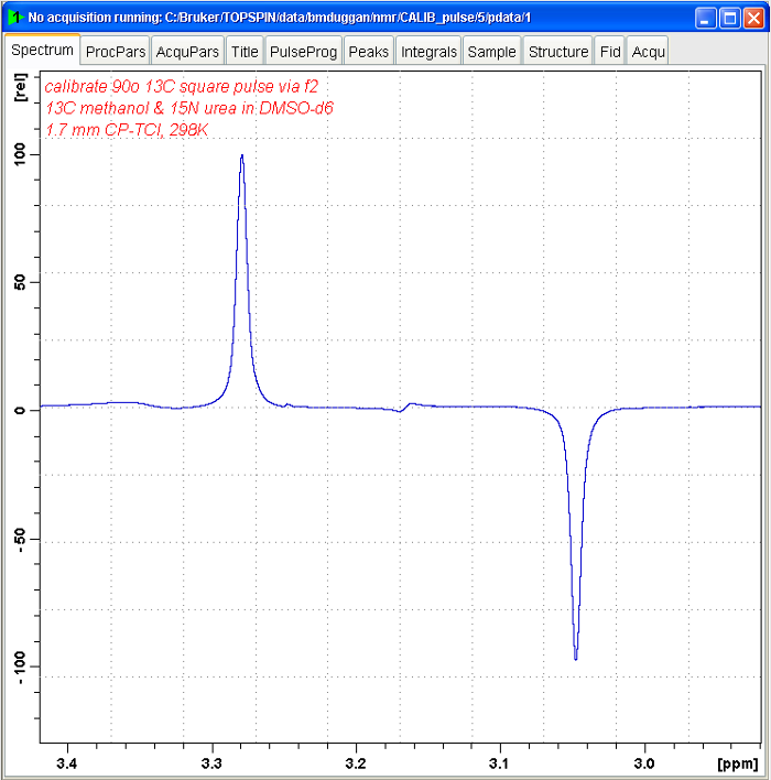
To calibrate the decoupler pulse using the pulse calibration standard a multipulse pulse program, decp90, is used. This consists of a 90o decoupler pulse that creates antiphase magnetisation followed by a 90o transmitter pulse that converts the antiphase magnetisation to unobservable double quantum magnetisation. If the inital decoupler pulse is exactly 90o then all of the magnetisation will be in the double quantum state during detection and no signal will be observed. The spectrum produced by the decp90 pulse sequence shows the 1H resonances split by the coupling to the heteronucleus. Since it is residual antiphase magnetisation that is detected the lines of the doublet are of opposite sign.
In practice the desired decoupler power level (PL2) is selected, an inital spectrum with a pulse length less than the 90o pulse is obtained, and then the pulse length is adjusted until minimal signal is obtained. The values of P3 and PL2 that give minimal signal are the 90o decoupler pulse length and attenuation that you will use in your experiments.
Preparation
Insert the standard pulse calibration sample into the magnet ("ij"), lock ("lock"), and read the decoupler pulse calibration parameters ("rpar UCSD_CAL_13C_DEC"). Load the default pulses and powers ("gpro"), tune and match the probe ("wobb"), and shim ("tsg").
You need to determine the high power 90o 1H transmitter pulse and attenuation for the pulse calibration sample using the method above.
Determine phasing
Set the decoupler pulse (P3) to a value less than the 90o pulse, say 2us, acquire an fid ("zg"), fourier transform ("ft") and manually phase correct. You need to have one peak of the multiplet positive and the other negative.
Determine accurate 90o pulse
Increase the value of P3, record another fid ("zg") and process it ("efp"). The two peaks should have decreased in intensity. Keep adjusting the value of P3 until the peaks are as small as possible. The value of P3 that gives minimal signal is the 90o decoupler pulse at the attenuation value (PL2) that you were using.
Calibrating 15N decoupler pulses
The method above describes how to calibrate 13C decoupler pulses. To calibrate the 15N decoupler pulse use the same method but read the 15N calibration parameter set ("rpar UCSD_CAL_15N_DEC"). This uses the pulse sequence decp90f3 in which the 15N 90o pulse that you will adjust is P21, and the attenuation is PL3.
Calculating pulses
Because our Bruker amplifiers have been calibrated and a correction table generated to linearise their response it is possible to calculate pulse lengths and attenuations from calibrated values. This simplifies determining power levels for TOCSY and ROESY spinlock pulses, for selective pulses in solvent suppression experiments and for heteronuclear decoupling.
Square pulses
To calculate the attenuation at another pulse length use the command "calcpowlev". "calcpowlev" will prompt you for the desired pulse length and the calibrated pulse length, then report how much to change the calibrated attenuation by. For example, if you want to determine the power level to use for a TOCSY spinlock you would enter the pulse length for the spinlock pulse (~28us), then the high power pulse length that you have calibrated (~10us). The macro will report the required change in the attenuation (8.94 dB) which you can add to the attenuation used for the high power pulse (4.0 dB) to get the attenuation for the spinlock pulse (4.0 + 8.94 = 12.94 dB).
To calculate the pulse length at another attenuation use the command "calcplen". "calcplen" works in a similar way to "calcpowlev", requesting the desired power level and a calibrated power level then reporting the pulse length at the desired attenuation.
Shaped pulses
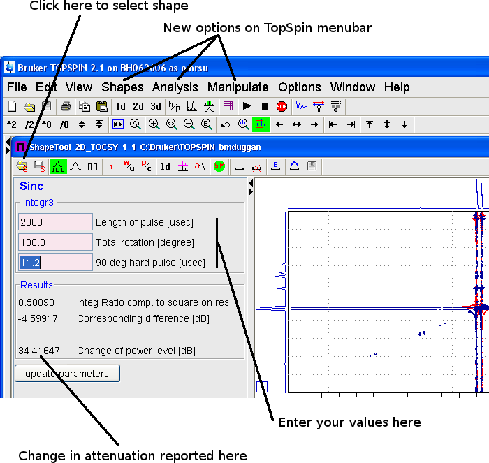
To calculate pulse lengths and attenuations for shaped pulses you can use shape tool. In TopSpin type "stdisp". A new window will appear with its own menubar along the top and the options along the top menu bar in the original TopSpin window will change. Click on the open folder icon then "Shape" to open a list of pulse shapes to select from.
If you select a non-adiabatic shape (e.g. Sinc.1000) you can calculate the attenuation for it by selecting Analysis -> Integrate Shape. The shape tool window will change to show three pink boxes where you must enter the length of the shaped pulse, the desired total rotation, and the length of the calibrated 90o high power pulse. Pressing the enter key after entering these values will update the enumbers reported under "Results". You need to add the reported "Change of power level" to the attenuation used for your calibrated 90o high power pulse.
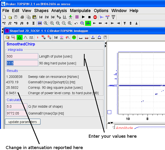
If you select an adiabatic shape (e.g. Crp60,0.5,20.1) you calculate the attenuation by selecting Analysis -> Integrate Adaibatic Shape from the TopSpin menubar. The window will change to show a panel on the left with two pink boxes in which you need to enter the pulse length, and the 90o high power pulse. Pressing enter updates the values reported under "Results". The change in attenuation should be added to the attenuation used for your calibrated hard 90o pulse.
Written by Brendan Duggan. Last modified 2022-Jul-22
Section 'Sub' Navigation: