
Acquiring Data
Insert sample tube into spinner
Make sure you use the correct spinner for your sample tube!
The 1.7 mm capillary tubes use a tall spinner with a tube that projects vertically above the widest part of the spinner. The 1.7 mm tubes simply drop into the spinner and hang by the cap. These tubes can be removed from the spinner by gently pushing them from the bottom until the cap emerges from the top of the spinner.
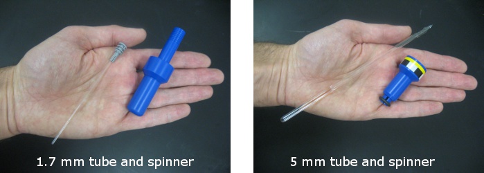
The 5 mm spinner is only half the height of the 1.7 mm spinner and is widest at the top. The spinner grips the 5 mm tube and prevents it from sliding up and down. The position of the 5 mm tube within the spinner needs to be adjusted using a depth gauge. If you have > 450 ul of solution in a 5 mm NMR tube you can gently push the tube down through the spinner until the tube contacts the bottom of the depth gauge. If you have less sample volume you will need to center the solution on the black marks representing the detection coils on the side of the gauge.
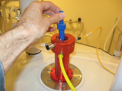
Put spinner with sample tube in magnet (ej, ij)
Turn on the air flow by typing “ej” in TopSpin. Wait until you can hear air flow through the central bore of the magnet. Place the spinner with the sample tube in the bore at the top of the magnet so that it floats in the air. You should feel resistance to downward pressure before letting go of the sample. Lower the sample into position in the magnet by typing “ij” in TopSpin. You should hear a clunk when the sample seats itself properly.
Lock onto solvent signal (lock)
In TopSpin enter the command “lock” and select your solvent from the window that pops up. If you cannot lock enter the command “rsh” and select a set of shims corresponding to the probe and your solvent, e.g. “tci_cdcl3”, then try locking again. If you still have problems locking check here.
Check temperature (edte)
If you are running long experiments such as 2Ds make sure the temperature is being maintained by typing “edte” in TopSpin. This will start a new window where you can set the temperature and air flow rate and monitor the temperature and heater power.
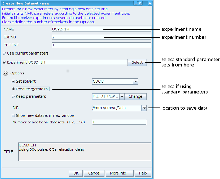
Create a new dataset (new)
In TopSpin type “new” to create a new dataset. In the window that pops up enter a name for your experiment, and an experiment number. It’s a good idea to use your sample name for the experiment name and different experiment numbers for the different types of spectra you will acquire on that sample. Choose either "Use current parameters" to copy the parameters of your current dataset to a new one, or click on "Select" to use one of the standard parameter sets.
Make sure the "Options" section is expanded. Check the "Set solvent" checkbox and select your solvent from the dropdown menu. If you are using a standard parameter set check the "Execute 'getprosol'" radiobutton. In the "Dir" dropdown menu select the directory you want to save your data to, or type it in if its not there. The "Title" box can be used to save some notes about the experiment.
Tune and match (wobb)
In TopSpin type “wobb”. The central window will change to display a curve that should dip towards the bottom of the screen near a central vertical red line. Check that you are running wobb on the desired nucleus in the text at the top right.

To tune and match the probe to your sample you have to adjust rods that project from the bottom of the probe. On the cryoprobes each nucleus has a pair of rods, one for tuning labelled "T", and one for matching labelled "M". The 1H rods are yellow, the 13C rods blue, the 15N rods red, and the 2H rods dark gray. The rods are adjusted by turning them with a tool that slips over the end of the rods and fits into the slots.
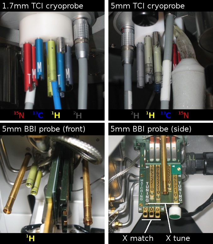
On the room temperature 5 mm BBI probe there is a pair of yellow rods for tuning and matching the 1H channel and brass sliders for the broadband channel. The brass sliders need to be adjusted to the frequency corresponding to the nucleus you wish to detect. A card attached to the probe gives the frequencies of some common nuclei. To adjust the sliders use the tool hanging from the probe by a metal chain. A knob on its end fits into a hole on the end of the sliders and lets you move them up and down.
Adjust the tuning and matching so that the wobb curve sharpens, is as low as possible, and lines up with the central vertical red line. Adjusting the tuning will move the dip sideways, while the matching will move it up and down and cause it to sharpen. Note that the matching interacts with the tuning, so you will probably have to go back and forth between the two. Once you are happy with the tuning and matching you can stop wobb by clicking on the stop icon at the top left, or by typing "stop" in TopSpin.
If you are running 1Ds of multiple samples in the same solvent tuning and matching need only be done for the first sample.
If you are running heteronuclear experiments it is best to start wobb in a heteronuclear experiment. This will allow you to tune all the nuclei you will be using. Wobb will start with the lowest frequency allowing you to tune and match that. To move to the next higher frequency click the stepup icon in the wobb window, or press F2 then F1 on the top of the preamplifier stack.
Shim (tsg)
Topshim can automatically gradient shim your sample. Type “tsg” in TopSpin. In the topshim window that pops up check that the "Optimise for" nucleus is the nucleus you will detect. (This is 1H for all experiments except 1D 13Cs and DEPTs where it is 13C.) To improve the off axis shims select “Z-X-Y-XZ-XY-Z” from the “after” dropdown menu in the “tune” section. Please note this is not tuning the probe. You need to use wobb to do that. Click on “Start” to start gradient shimming.
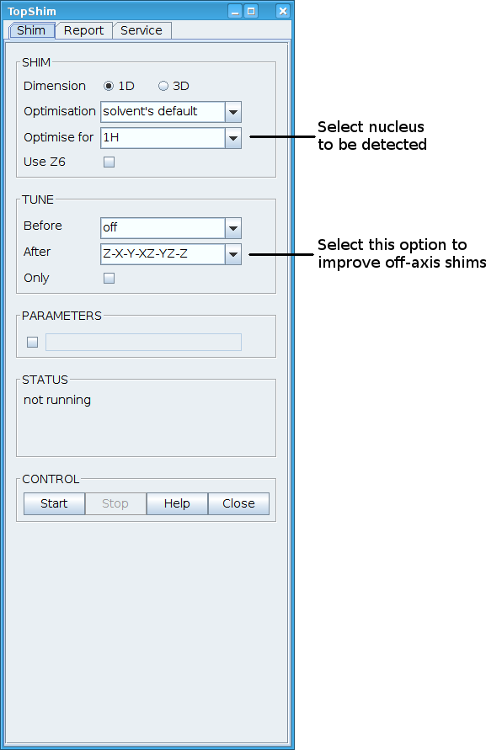
If your solvent is H2O you can select 3D shimming, but in most cases this should not be necessary. 3D shimming takes about 10 minutes compared to one to two minutes for 1D shimming.
After finishing shimming the “Report” tab of the topshim window will tell you the standard deviation of the B0 field inhomogenity before and after shimming. You should be able to get a B0 standard deviation of 0.50 Hz or less. Higher values indicate that the shimming is not very good. The report tab also reports the shims that it altered and the size of the change. If shimming fails error messages will appear on the “Report” tab.
Optimize parameters (rga, gs)
To get maximum sensitivity the receiver gain should be set to the highest value that does not clip the FID. In TopSpin type “rga” to automatically find the best value for RG. You should be able to get a value of at least 128 for RG.
Alternatively, you can use “gs”, a mode in which you can alter parameter values and monitor in real time the affect on the FID or fourier transformed spectrum. Entering "gs" will display a panel on the left listing parameters whose values you can change, and a panel on the right to display the FID or fourier transformed spectrum. To change parameter values use the tabs and radiobuttons in the left panel to select a parameter. The parameter's value can be altered by moving the slider or by entering values in the pink box. The sensitivity setting above the slider adjusts the size of the changes made with the slider.
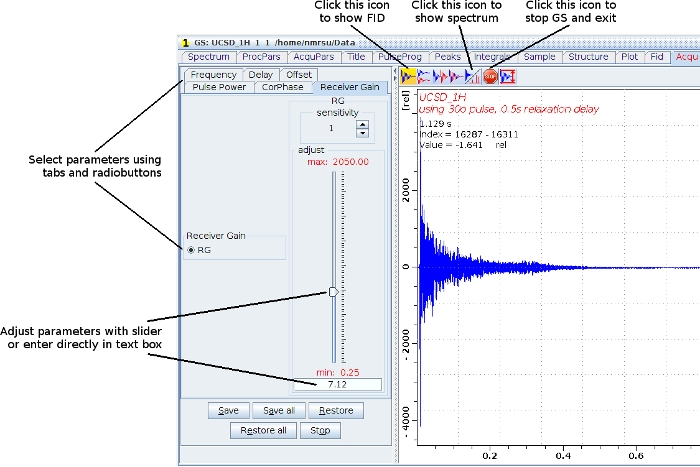
To optimize the receiver gain in "gs" mode, display the transformed spectrum and select the "Receiver Gain" tab. Use the slider to adjust the value of RG until the signals are as large as possible without wiggles appearing in the baseline.
Other parameters that are often adjusted using gs are; O1, the position of the center of the spectrum, which needs to be exactly on the water resonance for a water suppression experiment; PL9, the power with which the water resonance is saturated in a presaturation experiment; and shaped pulse power levels such as SP3 and SP1 in water flipback and excitation sculpting experiments.
To optimize the spectral width for your sample you need to adjust the sweep width ("SWH") and the carrier frequency ("O1"). To do this first collect a spectrum with a large sweep width so that all your peaks are observed. Next, use the cursor to zoom in on the region you want. Finally, click on the icon at the top right with a bent red arrow above a blue line. The values of SW, SWH, O1 and SFO1 will be modified to match your expansion. You may want to note the values of SWH and O1 that are reported in the popup window to use in other experiments.

Collect data (zg)
To start acquiring data type “zg” in TopSpin. This will overwrite any data you currently have in this dataset.
If you wish to run more than one experiment on the same sample there are two ways to do it. The command "multizg" will prompt you for the number of experiments to run, start acquisition in the current dataset, increment the experiment number, create the new dataset if it doesn't already exist, and start acquisition in the new dataset. It will repeat this until the requested number of experiments have been run. Setting up a series of datasets with the same experiment name and consecutive experiment numbers will allow you to run a series of experiments. It is also possible to queue up experiments with different experiment names, or to run them in a order different from the ordering of the experiment number, if you have selected "Enable automatic command spooling" under Options -> Preferences. With this option selected you can simply type "zg" in a series of datasets and the experiments will be queued in the command spooler.
Process data (ft, apk, xfb)
1D processing
- “ft” will fourier transform the FID.
- “ef” will apply an exponential window function to the FID before fourier transformation. The parameter LB defines in Hz the amount of line broadening used.
- “apk” will automatically phase the spectrum.
- “efp” will apply an exponential window to the FID, fourier transform it, and apply the previously determined phase correction to the spectrum.
- “abs” will do an automatic baseline correction.
- "tr" will transfer data from an acquisition buffer to a buffer where it can be processed. This is useful if you are running a long 1D e.g. a 13C, and want to process the data before acquisition is complete. Repeating the command adds the new data to what was previously transferred, and at the end of the experiment all the data is combined.
2D processing
- “xfb” will do a two dimensional fourier transform. It can be done at any time after the first slice of the 2D has been acquired and will use all the data currently available.
- "rser x” will read row x of the 2D data and allow you to process it as a 1D. This is useful for checking a 2D experiment is working properly if you don’t want to wait for more data to be collected.
- “clev” will calculate the best threshold level and the spacing between subsequent levels for optimal display of the 2D spectrum.
Written by Brendan Duggan. Last modified 2022-Jul-22
Section 'Sub' Navigation: